The n days of Christmas

A while ago, I read somebody write (probably on Twitter) that the Christmas song The Twelve Days of Christmas is a good way to teach students about quadratic growth, since the time required to sing the song grows quadratically as each verse increases its length. I thought this was great. But the more I thought about it, it started to bother me.

Grammatically, the song is not about what appears to be quadratic growth. In the song, the narrator’s true love gifts them one partridge on the first day, then another partridge in each subsequent day.

On the first day of Christmas, my true love gave to me a partridge in a pear tree.

On the second day of Christmas, my true love gave to me two turtle doves and a partridge in a pear tree.

The narration does not say that the partridge on the second day is the same partridge that was given on the first day. So my interpretation of this is that the narrator, by day two, has now collected two partridges. This changes things.

The question that I’ve been trying to figure out is what the growth rate is for the total number of gifts (where some of these gifts are humans, so that’s weird…) on the $n$ th day of Christmas. Let’s assume for the sake of making the math interesting that the number of days of Christmas grows toward infinity.

They key is that on the $i$ th day of Christmas, a new gift is introduced. This gift will be given in groups of $i$ each day from then on. For example, for $i=1$ , the partridge is introduced, and each subsequent day, the true love gives one more partridge. For $i = 2$ , the turtle doves are introduced, and the true love gives 2 turtle doves each day for the rest of eternity. Another key point is that these gifts don’t start until the $i$ th day.

This pattern means that on the $n$ th day, the narrator owns $i(n - i + 1)$ of the $i$ th gift. That’s a fairly straightforward linear growth. But my main question is how many total gifts does the narrator have on day $n$ ?

The formula here is
$f(n) = \sum_{i=1}^n i (n - i + 1)$ ,
which we can simplify by massaging the equations as follows
$f(n) = \sum_{i=1}^n in - \sum_{i=1}^n i^2 + \sum_{i=1}^n i = n \sum_{i=1}^n i - \sum_{i=1}^n i^2 + \sum_{i=1}^n i$ .

These summations now have some well known formulas. Using the power of my computer science education (and Wikipedia), this formula simplifies to
$f(n) = n \frac{n(n+1)}{2} - \frac{n(n+1)(2n+1)}{6} + \frac{n(n+1)}{2}$ .
Some more massaging leads to
$f(n) = (n + 1) \frac{n(n+1)}{2} - \frac{n(n+1)(2n+1)}{6}$ .

It’s looking like it’s cubic growth. But let’s finish to make sure. We can combine fractions now, leading to
$f(n) = \frac{3n(n + 1)(n+1)}{6} - \frac{n(n+1)(2n+1)}{6} = \frac{3n(n+1)(n+1) - n(n+1)(2n+1)}{6}= \frac{1}{6} (n^3 + 3n^2 + 2n)$ .

Thus, the total number of gifts received by the narrator is $\Theta(n^3)$ .

Merry Christmas and Happy Holidays!

A Small Puzzle about Saddle-Point Optimization

Here’s a little problem I’ve been wondering about for a while. Suppose you’re trying to find the solution to the saddle-point optimization
$\min_{x} ~ \max_{y} ~ f(x) + g(y) + x^\top M y$ ,
where $x$ and $y$ are vectors, functions $f$ and $g$ map from their respective vector spaces to scalar outputs, and $M$ is a matrix. Assume that $f$ is convex and $g$ is concave. Let’s call the objective value of this problem $L(x, y) = f(x) + g(y) + x^\top M y$ .

Suppose that some oracle gives you a functional
$h(x) = \arg\max_{y} ~ g(y) + x^\top M y$ ,
i.e., the solution to the inner maximization of the original saddle-point problem $\arg\max_y L(x, y)$ . We can then consider the optimization
$\min_x ~ L(x, h(x)) = \min_x ~ f(x) + g(h(x)) + x^\top M h(x)$ .

There’s a surprising (to me) result that the gradient of the function $L(x) \equiv L(x, h(x))$ is
$\nabla_{x} L = \nabla_x f + h(x)^\top M^\top$ .

This gradient somehow ignores the gradient of $h(x)$ , which is clearly a function that depends on $x$ . This gradient also happens to be the partial gradient with respect to $x$ . Why does the dependence on $y$ disappear? Let’s try to see why this is true.

Before we do that, let me give an example of where this form of optimization arises. The most prominent example is for Lagrangian relaxation. When you’re trying to minimize some function $J(x)$ with a constraint $Ax = b$, you can form the Lagrangian problem
$\min_x ~ \max_y ~ J(x) + y^\top (Ax - b)$ ,
which takes the general form we started with if $f(x) = J(x)$ , $g(y) = -y^\top b$ , and $M = A^\top$ . This general form also arises in structured prediction, for example when the inner maximization is the separation oracle of a structured support vector machine or the variational form of inference in a Markov random field.

Back to the general form, let’s try taking the gradient the traditional way, starting with
$\nabla_x L = \nabla_x f + \nabla_x g(h(x)) + \nabla_x x^\top M h(x)$ .

The second term can be expanded with some chain rule action:
$\nabla_x g(h(x)) = \underbrace{\left(\frac{d~g(h(x))}{d~h(x)}\right)}_{1 \times |y|} \underbrace{\left(\frac{d~h(x)}{d~x}\right)}_{|y| \times |x|}$ . (I’m probably botching the transposes here.)

The third term can be expanded with product rule:
$\nabla_x x^\top M h(x) = h(x)^\top M^\top + x^\top M \left(\frac{d~h(x)}{d~x}\right)$ .

We also know something about $h(x)$ . Since it comes from maximizing $L$ , we know that its gradient wrt $y$ is zero, i.e.,
$\nabla_y L(h(x)) = 0$ ,
which means $\nabla_{h(x)} g(h(x)) + x^\top M = 0$ , and $\frac{d ~ g(h(x))}{d~h(x)} = - x^\top M$ .

The second term then can be replaced with
$\left(\frac{d~g(h(x))}{d~h(x)}\right) \left(\frac{d~h(x)}{d~x}\right) = - x^\top M \left(\frac{d~h(x)}{d~x}\right)$ .

This replacement directly cancels out a term in the product rule (third term). Leaving us with
$\nabla_x L = \nabla_x f - x^\top M \left(\frac{d~h(x)}{d~x}\right) + h(x)^\top M^\top + x^\top M \left(\frac{d~h(x)}{d~x}\right) = \nabla_x f + h(x)^\top M^\top$ .

I suspect there’s an even more generalized form of this property, perhaps generalizing the bilinearity of the problem to some other kind of convex-concave relationship between $x$ and $y$ . Let me know if you know of anything along those lines.

Announcing the wish☁cloud

This spring, I spent some time on a hobby project that has been on my back burner for over a decade. This project is unrelated to my research or anything I do in my day job (aside from being practice for building web apps, which may be useful for my research eventually). The project is called the wish☁cloud.

What is the wish☁cloud?

The wish☁cloud is a social web application where users can vicariously fulfill their wishes. Users post things that they wish they could do or experience, and other users realize these wishes for the original wishers. The intent is to use technology to amplify the shared human experience, giving its users little moments of happiness and gratitude.

The history of the wish☁cloud

The wish☁cloud began as a class project from a course I took in college on the role of the Internet in society. Back then, in 2004, it was called “Seriously Vicariously.” Since then, I’d been waiting to build it, or hoping someone else would scoop the idea so I could take part in it.

A confluence of factors led me to finally build a prototype for the wish☁cloud this spring: I’d been thinking a lot about the role of the Internet in our lives and been missing the optimism that existed during the early days of the social web; I’ve been wanting to learn modern web programming to hone my skills; and I needed a hobby project to take breaks from academic life and maintain my sanity. Thus, the wish☁cloud now exists in a nascent form.

How can I play on the wish☁cloud?

Now that I’ve built it, I want to see if it can actually support users. Check it out at http://wishcloud.org. ~~There’s not much there yet.~~

~~If you’re interested in getting an account and trying it, fill out this form: https://goo.gl/forms/oT0Kk8m8D97hVTga2~~

I’ll send out invitations at my discretion as I gain more confidence that the site works as I intend it to. It may be a while as I’m working out a few issues, and I won’t have much hobby time during the end-of-semester crunch. But add your name if you’re interested!

Edit: I’ve opened up the service to anyone who wants to sign up. I recommend signing up with an external account so that my server isn’t storing any login credentials. You can revoke access to your social media login at any time.

I suspect it will run into problems quickly since I’m not an expert in web programming, system administration, or basically anything behind the entire wish☁cloud. I hope that when it works, you have fun and find a little happiness on the site.

How I prefer students address me

A few students have asked me lately how I prefer to be addressed. Here’s an ordering of my preference.

Bert
Professor Huang
Dr. Huang
Dr. Bert
Professor Bert

I’m cool with any of these. I get Dr. Huang most often, for some reason. That’s okay. I’m not sure why I don’t like that as much as Bert or Prof. Huang. It’s probably because being a university professor is my dream job and if you’re gonna be formal, you might as well remind me that I’m doing my dream job (especially right before you ask me to do something I probably don’t want to do). And I like first name because, as a computer scientist, all my favorite professors who I looked up to during my career have been cool first-name people.

But no big deal. You can also just call me “hey you,” or nothing.

Just don’t call me Mr. Huang.

Machine Learning’s Poor Fit for Real Data

There’s a growing sentiment out there with all the wonderful things happening in artificial intelligence, machine learning, and data science that these technologies are ready to solve all the things (including how to kill all humans). The reality is there are still a bunch of significant hurdles between us and the AI dystopia/utopia. One big one that is the main impetus behind my research is the disconnect between the statistical foundations of machine learning and how real data works.

Machine learning technology is built on a foundation of formal theory. Statistical ideas, computer science algorithms, and information-theoretic concepts integrate to yield practical methods that analyze large, noisy data sets to train actionable and predictive models. The power of these methods has caused many to realize the value of data.

Yet, as data collection accelerates, weaknesses of existing machine learning methods reveal themselves. The nature of larger-scale data collection violates key assumptions in the foundation that made machine learning so effective. Most notably, statistical independence is no longer achievable with large-scale data. Data is being collected from highly interacting, entangled, complex systems. Human data describes people interacting in a single global social network; ecological data represents measurements of organisms inhabiting complex, shared ecosystems; and medical data measures the interconnected, biological systems that govern health.

Origins in Experimental Statistics

The concept of statistical independence is a natural fit for laboratory experimentation. In laboratory experiments, scientists test hypotheses by running repeated experiments in closed environments. By design, the measurements taken during each experiment are independent. Because one experiment can’t affect another’s result, classical statistics can confidently quantify the effects of factors in the experiment, even in the presence of randomness.

For example, a typical pre-clinical laboratory drug trial would use a population of animal subjects, administering a drug to part of the population and giving no treatment to a separate control subpopulation. The two subpopulations would be managed to ensure that confounding factors, such as genetics, are equally distributed. The individual subjects would be kept separated in isolated environments. By preventing subjects from interacting with each other, any observations of the drug’s effects can be considered fully independent samples, and classical statistics would enable comparison of effects with quickly converging confidence intervals.

In modern data, measurements are taken from “the wild.” Modern data is analogous to a version of the experiment where the animal subjects interact, sharing food, contact, and communication. Generally, data collections describe large populations of interacting parts, with each measurement related through correlated paths. As modern data collection technology becomes faster and cheaper, the data necessarily becomes increasingly interdependent.

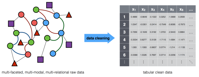
Illustration of the data cleaning task. A common view of complex data is that it can be “cleaned” to fit the structure expected in classical statistics and machine learning methods. But this cleaning typically decimates the nuanced information present in data from real-world, complex phenomena.

The Myth of Clean Data

It’s tempting to interpret these nuances of real-world data to be simply nuisances. One may attempt to convince oneself that the discrepancy between classical statistical methods and real data can be remedied by data cleaning. Data cleaning—a key skill in modern data analysis—involves taking raw data, processing it to remove spurious outliers, undesired dependencies, and biases created by interacting measurements, then performing supposedly clean analysis on the supposedly clean data.

The clean data concept encourages deliberate omission of information, introduction of unjustified assumptions, and fabrication of facts, to turn real-world data, with all its complexities, into rectangular tables of independent samples. These manipulations undo many of the virtues of data-driven thinking.

The perception that machine learning methods require such destructive preprocessing is a major failure in the technology transfer from machine learning research to practical application. And the reasons for this failure manifest in the various costs associated with more nuanced machine learning methods. Methods that can reason about interdependent data require more computational cost—the amount of computer time and energy needed to learn, reason, and predict using these methods—and cognitive cost—the amount of expertise necessary to apply, understand, and interpret these methods.

“Conclusion”

So what’s the point of my arguments here? I’m not super certain, but here are a few possible takeaway points:

Big data is complex data. As we go out and collect more data from a finite world, we’re necessarily going to start collecting more and more interdependent data. Back when we had hundreds of people in our databases, it was plausible that none of our data examples were socially connected. But when our databases are significant fractions of the world population, we are much farther away from the controlled samples of good laboratory science. This means…
Data science as it’s currently practiced is essentially bad science. When we take a biased, dependent population of samples and try to generalize a conclusion from it, we need to be fully aware of how flawed our study is. That doesn’t mean things we discover using data analytics aren’t useful, but they need to be understood through the lens of the bias and complex dependencies present in the training data.
Computational methods should be aware of, and take advantage of, known dependencies. Some subfields of data mining and machine learning address this, like structured output learning, graph mining, relational learning, and more. But there is a lot of research progress needed. The data we’re mostly interested in nowadays comes from complex phenomena, which means we have to pay for accurate modeling with a little computational and cognitive complexity. How we manage that is a big open problem.

Inner dual methods for structured output learning

One of the big challenges in making structured predictors more practical is that they can be really slow compared to ~~the hack of assuming your variables are independent~~ unstructured models.

There’s a line of research that partially addresses this expensiveness by avoiding repeated inference during the learning phase. I call it “inner-dual learning,” but it goes by many names.

The basic idea is that we do prediction by solving an optimization problem

$\arg\max_x f(x; \theta)$ .

For example, the objective $f$ could be an energy and an entropy, which would make this optimization related to variational marginal inference in probabilistic models, or it could just be a linear objective over a structured output space, which is typical in combinatorial structured prediction. For various reasons, we often solve these inference objectives using a dual version of the inference optimization

$\arg\min_\alpha g(\alpha; \theta)$ ,

where

$\min_\alpha g(\alpha; \theta) = \max_x f(x; \theta)~\text{and}~g(\alpha; \theta) \ge f(x; \theta), \forall x, \alpha$

The learning optimization often takes the form of

$\min_\theta ~ R(\theta) + \max_x f(x; \theta) + \text{something}$

which is a saddle-point problem minimizing over parameters $\theta$ and maximizing over the predictions $x$ . The “something” is typically a function of $\theta$ that doesn’t depend on $x$ .

The standard way to solve saddle-point-y things like this is to repeatedly

solve the inner inference optimization,
take the (sub)gradient with respect to the parameters $\theta$ , and
update the parameters using your favorite gradient-based optimization routine.

Having to solve the inference for each gradient step is painful, especially when you’re dealing with complex structured outputs. So the inner-dual idea is to replace that inner maximization with a minimization of its dual. (For real duals of concave functions, this forms an upper bound on the original learning objective!)

$\min_{\theta, \alpha} R(\theta) + g(\alpha; \theta) + \text{something}$ .

The problem then becomes a joint minimization over the parameters and the dual variables! Moreover, we often have very fast message-passing style algorithms for solving the dual minimization. That means we can, in a principled way, interleave learning and inference, rather than using one as a subroutine for the other. The learning loop then becomes

make a single-pass update to the inner inference dual variables (e.g., pass messages),
take the (sub)gradient of the dual objective with respect to the parameters $\theta$ , and
update the parameters using your favorite gradient-based optimization routine.

As far as I know, the first such inner-dual method was done in the seminal paper by Ben Taskar and folks at ICML ’05 (link). That paper is really well cited and has been read by tons of people, but seemingly few have picked up on this trick. Instead, I usually see it cited for the primal structured-output learning objective they introduced, which has been the foundation of a lot of related work. Part of the reason for the lack of recognition for this idea is that Ben et al. formulated the dual as a quadratic program that had to be passed into a general-purpose quadratic programming tool, which I imagine is super slow.

Years later in 2010, Ofer Meshi and folks (link), and Tamir Hazan and Raquel Urtasun (link) used the same idea but using the dual objectives from fast message-passing algorithms for graphical model inference as the inner dual. Later on in 2012, Alex Schwing and folks (link) used this for latent variable modeling, also using message-passing duals. In 2015, in work with Stephen Bach, Jordan Boyd-Graber, and Lise Getoor, we used the inner dual method twice to even more aggressively dualize expensive inferences during latent variable learning (link). We did this specifically for hinge-loss MRFs and with ADMM inference, but I’m working with my current students on extending this to be more general now. Also last year in 2015, Chen, Schwing et al. revisited the inner dual idea to train deep models with structured predictors attached to them (link).

I’m sure there are other examples of this trick in the literature, though one problem with finding it is that it hasn’t been consistently named. Both the Taskar and Hazan (et al.) papers don’t really give it a name, referring to the idea as just a dual objective; Meshi et al. refer to the idea as using a dual loss; Bach and I referred to it as inner dual (or in our case, since there were two dual inferences for latent variable learning, we called it paired dual learning); and Chen/Schwing et al. called it blending inference and learning. My preference is inner dual, as should be obvious by how I refer to it throughout this post. I think it captures the fact that we’re using the dual objective of the inner optimization. But pay attention for these other names of it!

While inner-dual methods seem to do a great job of alleviating the computational cost of learning, they still train models that are expected to run expensive inference at test time. That’s not great. There are related lines of research on training structured predictors that will do something cheap at test time, like truncate a message passing optimization, but it remains to be seen how to integrate these different approaches without nullifying their benefits.

Scientific Hypothesis: We are the Best

It’s reviewing season for the summer conferences, so here’s something that’s on my mind as I’m doing my reviews.

One crappy thing that happens a lot in machine learning research is that researchers do non-scientific things like over-claiming, taking ownership, and bad experiment design. We end up with paper after paper, each claiming to present the best method with cherry-picked experiments that only demonstrate that the authors can draw prettier curves than other authors.

Sometimes authors use phrases like “our method” a lot in their description of the approach they’re demonstrating. Sometimes I even see tables or plots describing the final results from experiments where the legend entries are “our method,” “So and so’s method,” “SVM,” etc. This type of naming hints at a lack of objectivity.

Naming the proposed method is usually better, especially when the name actually describes the thing (so not an acronym that uses a letter from the middle of one of the words… c’mon people). Then the authors become scientists trying to understand the properties of some approach they discovered. And yes, they still get credit for discovering it, they just get fewer eye rolls.

This attitude also encourages poor experiment design. As computer scientists, we should want to understand the behavior of certain algorithms, so really good experiments would test many hypotheses about how the new algorithm performs under different conditions. We want to understand the strengths, weaknesses, and tradeoffs in comparison to other known methods. But many experiments in papers only test one hypothesis: “our method is the best method ever and you should purchase it.”

This problem is bad enough that I almost never trust the results of experiments in papers, or I always just think of them as synthetic sanity checks, even when they are using real data.

I’m certainly also quite guilty of this unscientific attitude and behavior. It’s very hard to avoid. On one hand, as scientists, we want to advance the world’s knowledge on machine learning, but on the other hand, as people who do science for a living, we want credit for advancing the world’s knowledge. That often leads to our papers reading more like patent applications than descriptions of scientific discovery. Yuck.

In conclusion, I’ve pointed out an annoyance and proposed no great solution for it. So I guess this qualifies as just ranting. But my method of pointing out this problem improves upon the state-of-the-art method by so-and-so et al. by 11%.

On Rejection and Acceptance Rates

A while ago, I posted about the emotionally difficult challenges of research. I mentioned half-jokingly at the end of that post that I would in the future write a post about another challenge: rejection.

Since some of the students in my group just submitted their first papers to the peer review process, I figured I’d actually go through with that plan now. We just submitted three papers to the KDD research track, which, when I last checked, has an acceptance rate of just under 20%. That means a few things. In expectation, 0.6 of my group’s papers will be accepted, and the MAP estimate (and marginal decoding) of how many papers will be accepted is zero.

Of course, the actual likelihood of acceptance or rejection is dependent on the quality of the work, but as we’ve seen recently from, e.g., the NIPS experiment, paper quality doesn’t have as certain an effect as we’d hope. What makes a scientific contribution worthy of acceptance is a very subjective concept, so even the best papers have a chance of landing some reviewers who just won’t be convinced.

So given these realizations, when submitting work for peer review, one must be somewhat prepared for rejection. It sounds easy, right? We know acceptance rates are low; we know it’s not personal; we know the reviewers that decide our fates are doing the best they can with very limited time. If we were perfectly rational, logic-based beings, there’d be no problem here. Just keep improving your work and trying again and again.

Of course, we aren’t purely rational and logical. Being rejected is one of the most difficult and painful parts of a researcher’s life. It genuinely hurts. As scientists, we want to be rational about it, but the visceral reaction to reading “we regret to inform you” comes with a plethora of painful emotions, from disappointment and sadness, to fear and anger.

The reason I thought it might be useful to write a post like this is similar to that of my previous post inspired by the TED talk. Scientists are often trained to ignore these emotions. We don’t talk about them much. We often try to only discuss the rational, actionable parts of rejection. “Use the feedback, and make the research better.” But the reality for me is closer to “get feedback, feel terrible, doubt yourself, blame system, blame yourself, briefly consider quitting, feel embarrassed for having these reactions, seek support from non-scientist friends and family, get back to work pretending you’re not hurt, eventually really get back to work.”

This whole ordeal is invariably part of the job. But like the emotional challenge of facing uncertainty and “the cloud” in research, it would be helpful to acknowledge that it is okay, normal, and expected to have these emotional reactions. That doesn’t preclude the more rational advice I’ve seen around, but I’d like not to perpetuate the fantasy that we can be perfectly rational about this whole process.

Eventually, once we realize that these emotions are normal, perhaps then it will be easier to filter them. Then we can find which emotions are useful, and work toward getting the ones that are not useful (i.e., most of them) out of our systems. Perhaps knowing that these emotions are a shared experience can help us manage them more easily.

Upcoming AISTATS paper

In about a week, our paper Unifying Local Consistency and MAX SAT Relaxations for Scalable Inference with Rounding Guarantees by Steve, me, and Lise will appear at AISTATS in San Diego. (Steve will be giving a talk on it Monday morning.)

The paper title is a mouthful, and it includes a pretty technical result, so here’s a weak attempt at explaining the intuition and take-away messages.

The paper is about MAP inference, or finding the most likely state in a probability distribution. Specifically, it’s about MAP inference in what we are calling logical Markov random fields (MRFs), which are MRFs whose potentials are defined by weighted logical clauses of a particular form. We show equivalences between two different approaches (and a third bonus one) for approximating MAP inference in these logical MRFs. These equivalences are theoretically interesting, but at least as importantly, they allow us to get the benefits of each approach, leading to fast MAP approximations that have constant-factor approximation guarantees.

What’s special about logical MRFs is that MAP inference is equivalent to finding the maximum weighted satisfying assignment to the logical variables, aka the MAX SAT problem. On the surface, this equivalence doesn’t seem exciting, because it equates one NP-hard problem to another. What makes it exciting is that there are some nice approximation algorithms for MAX SAT with quality guarantees, and these algorithms can therefore be applied to get quality guarantees for MAP. Unfortunately, the approximation method by the famous computer science duo, Michael Goemans and David Williamson, requires solving a linear program (LP) that scales not-so-well in practice, when using off-the-shelf linear programming algorithms.

Another approach for approximating MAP inference borrows from recent developments on doing fast inference in MRFs using local-consistency relaxations. At a very high level, these approaches relax the space of possible marginal probabilities (i.e., the marginal polytope) to a simpler space that only requires local consistency between marginal probabilities of variables and factors (i.e., the local marginal polytope). By solving the corresponding optimization over this simpler, relaxed set of constraints, many very fast message-passing algorithms have been discovered in the past few years. So it’s natural to try to use one of these local-consistency relaxation message-passing algorithms to do MAP inference in a logical MRF.

The main result we show in the paper is that these two seemingly different approaches are equivalent. This equivalence means that when we use these fast-in-practice local-consistency relaxation algorithms that pass messages to quickly find an approximate solution, we’re also able to get the solution to the linear-program subproblem of the MAX SAT approximation algorithm. Using the LP solution, we can perform a special rounding scheme that guarantees a constant-factor approximation.

The last bonus equivalence is that both of these approaches are also equivalent to the linear form of a hinge-loss Markov random field, which we’ve been studying over the past few years as a powerful class of probabilistic models with efficiently optimizable energy functions. The conversion from logic to hinge-loss MRFs (i.e., the principles behind probabilistic soft logic) had previously been motivated by connections to fuzzy logic, and now we have these other relationships to MAX SAT relaxation and local-consistency relaxation.

Behind the scenes, this last bonus piece is how we happened to find these equivalences. We initially were working with these hinge-loss MRFs and we had thought that these other approaches to doing inference in logically-defined MRFs seemed so different, that it’d be interesting to compare them. So we ran a few tests and discovered they were behaving similarly… very similarly; they were returning solutions with differences that were small enough to be numerical errors. This surprising behavior led to confusion, derivations, and finally understanding.

Finally, the super weird part: any (nondeterministic factored) discrete MRF can be converted to an equivalent logical MRF. This, in some sense, means the constant-factor quality guarantees that come from the equivalence between logical MRF inference and MAX SAT, also apply to any discrete MRF. But along the way of converting a discrete MRF to the restricted logical MRF form, the strength of this constant-factor guarantee must be weakened, especially since we know that MAP can’t be approximated to a constant factor unless P = NP. But it’s still an open question how this all fits together. Check out the paper, and maybe we can brainstorm about this in San Diego.

My Spring Conference Reviewing Data

Last night, I finally finished a marathon month+ of reviewing for machine learning and machine-learning-adjacent conferences. Because of my own poor calendar organization, I foolishly agreed to join the program committees for IJCAI 2105 (Machine Learning Track), KDD 2015, ICML 2015, and UAI 2015. These conferences all had reviewing periods during the month of March and this first bit of April.

My paper assignments for these conferences were six for IJCAI, five for KDD, six for ICML, and five for UAI. While I was reviewing these 22 papers, I was recording my initial overall recommendation (prior to discussion and author response) for each of these papers, just to measure how I tend to score papers. I figured I’d post some of these recordings here, with the major caveat that these are still tiny sample sizes and they are heavily biased by what papers and topics I like to bid on. I’m also going to convert all scores to a scale of [strong reject, weak reject, weak accept, strong accept] to both simplify and muddy up my data a bit to prevent any chance of some smartypants somehow de-anonymizing based on my silly blog post.

For IJCAI, my recommendations for my six papers were one reject, one weak reject, three weak accepts, and one strong accept.
For KDD, my recommendations for my five papers were three rejects, one weak reject, and one strong accept.
For ICML, my recommendations for my six papers were two weak rejects, three weak accepts, and one strong accept.
For UAI, my recommendations for my five papers were two rejects, two weak rejects, and one weak accept.

Overall, I recommended four rejects, six weak rejects, eight weak accepts, and three strong accepts. I gave zero strong reject recommendations. If my initial vote was the only one that counted, my accept rate for each conference is 66% for IJCAI, 20% for KDD, 66% for ICML, and 20% for UAI. Overall, my acceptance rate was a rather high 45%.

So what is the takeaway message? I’m not sure. I guess this still isn’t enough data to really tell anything. Let me attempt to make some claims.

The numbers suggest that I like ICML and IJCAI papers better than UAI and KDD papers. I would be pretty surprised if this is true and not just a result of randomness. It’s hard to tell with the IJCAI ML track being a brand new idea. I usually imagine myself as liking UAI papers the most of all the medium-sized ML conferences.
The numbers suggest that I like ICML papers about graphical models, structured prediction, and relational learning. Since these are the topic areas I usually bid on and that Toronto Paper Matching usually assigns to me. This is plausible, but not consistent with my low accept rate for UAI.
By a similar argument, the numbers suggest that I don’t like KDD papers on graph mining and relational models. This is also plausible, but surprising. I think in this case, I really like the problem area of data mining from complex network data, but maybe I’m often unsatisfied by the methods people propose. It’s possible I’m too critical of this kind of work.

Sorry these are all pretty weak analyses. The sample size is just too small. If I want to understand my own biases better, I need to volunteer to review even more (note to self: do not do this), or keep better records from previous years of reviewing.

Only one thing is absolutely clear from this month of reading all these submissions: seriously everyone needs to stop using the word “employ.”